Methods

Structure

1. Read in ssh

• remove anomaly
• detrend
• Filter

One point for each flow chart

This algorithm was developed with the main idea of decomposing oceanic Kinetic Energy into processes. Even when its implementation can be useful in multiple applications, the current version of the algorithm is primarily focused on methods to extract energy from SSH fields. However, according to few tests, it could be implemented to track eddies in pressure levels, isopycnals and even vorticity.

The criteria ranges were defined using a repetitive Southern Ocean simulation, particularly this section of the documentation was done analysing a section of the Aghulas current. For a detailed - code description, refer to how_it_works.ipynb

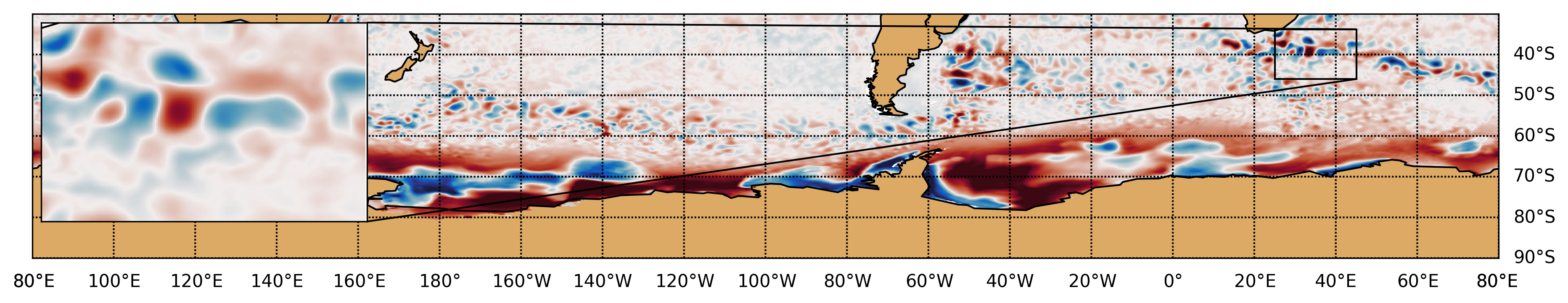
Figure 1. Section of the Aghulas current used to explain how the algorithm works.

Eddy Identification Criteria

TrackEddy identifies eddies when their outer most contours can be fitted by an ellipse (A. Fernandes and S. Nascimento, (2006)), the area of the eddy contour is smaller than \(2 \pi L_r\) (Klocker, A., & Abernathey, R. (2014)), the eccentricity of the fitted ellipse is smaller than \(\frac{b}{2a}\) and the field profile along the minor and major axis of the fitted ellipse must adjust to a Gaussian. Optionally, an additional criterion is implemented when the 2D Gaussian fitting is allowed, this criterion identifies eddies only if the fitted 2D Gaussian correlates over 90%. For additional information, please refer to the following subsections.

These criteria allows eddies to contain multiple local extreme values, which is particularly beneficial when they merge, interact or form from jets or other processes.

Ellipse Fitting

According with Fernandes (2006) an eddy can be represent as an ellipse. Therefore, in this algorithm the optimal ellipse is fitted to any close contour and in order to determine if it corresponds to an eddy, the correlation between the fitted ellipse and the close contour should be within the interval (\(e\)) :

\[0.85 < e \leq 1\]

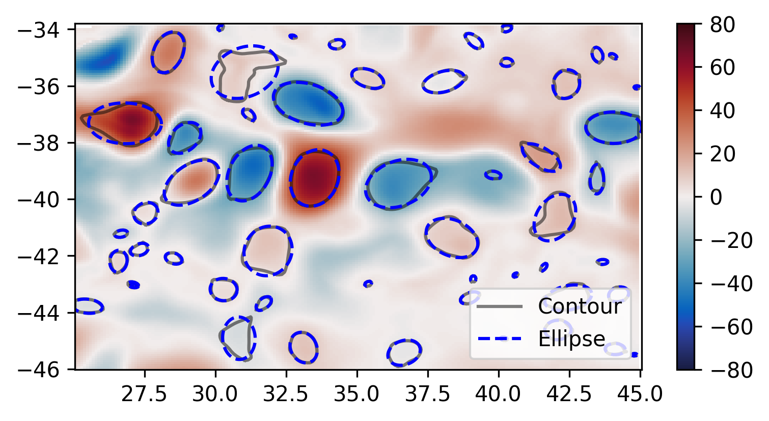
Figure 2. Identified contours only within the ellipse fitting interval (Ignoring any additional criteria).

Values around \(1\) represent an exact fitness and the minimum value accepted should be higher than \(0.85\).

Area Check

The eddy area (\(A_{eddy}\)) was defined as a box with sides of two semi-minor axis and two semi-major axis of the fitted ellipse. Klocker, A. (2014) proposed that the eddy length scale (\(L_{eddy}\)) is always smaller than two \(\pi\) Rossby Radius.

Therefore, the area of any identified eddy should be less or equal to a square with sides two times the Rossby Radius.

\[A_{eddy} \leq \left(2\pi \frac{(g'D)^\frac{1}{2}}{f}\right)^2 = \left(2\pi Lr \right)^2\]

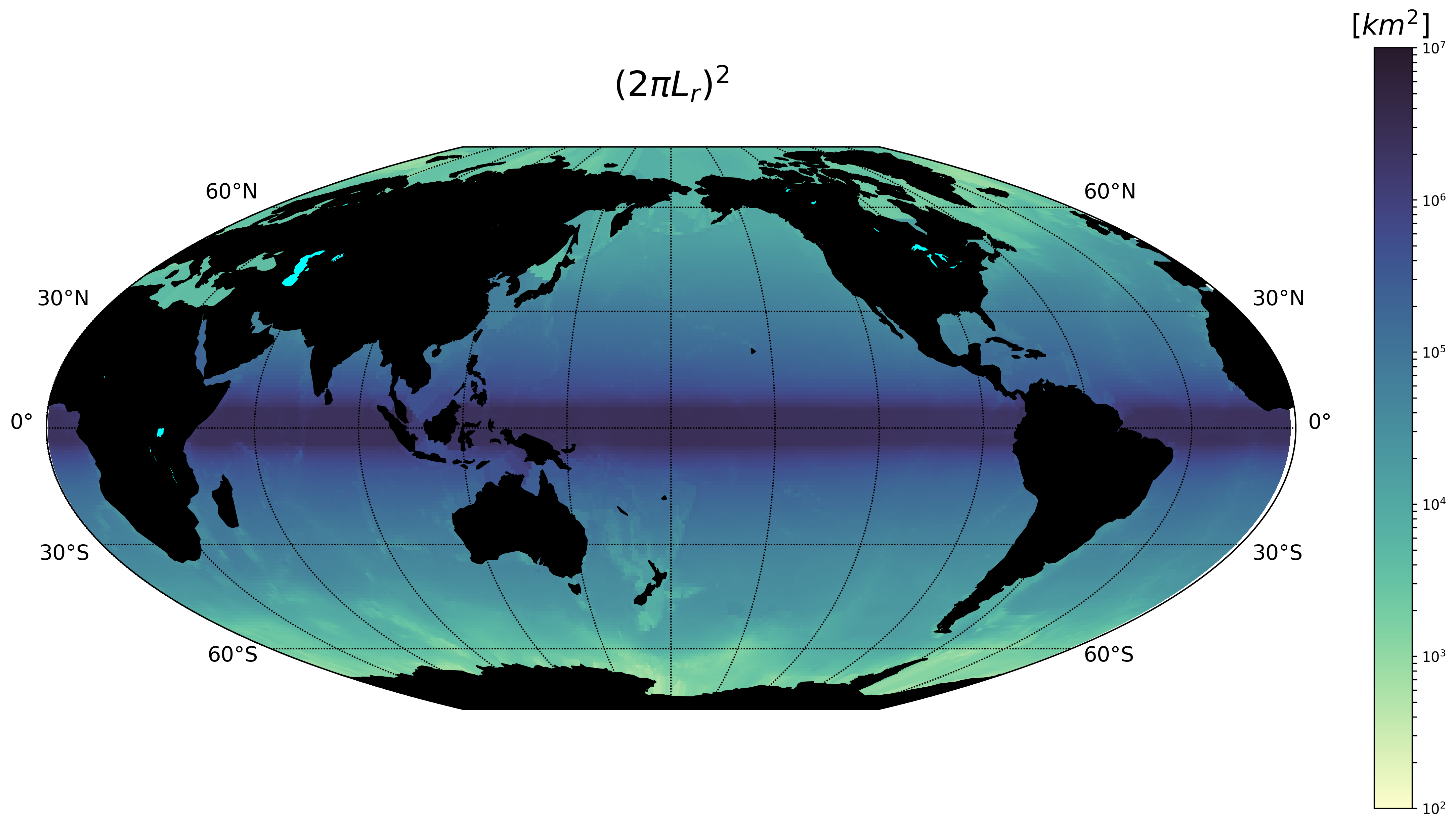
Figure 3. Global eddy area based on the First-Baroclinic Rossby Radius of Deformation.

Note

The Rossby Radius was obtained from the Global Atlas of the First-Baroclinic Rossby Radius of Deformation (Click here). Where values were inexistent, they were replaced by the closest known value (Fig. 3).

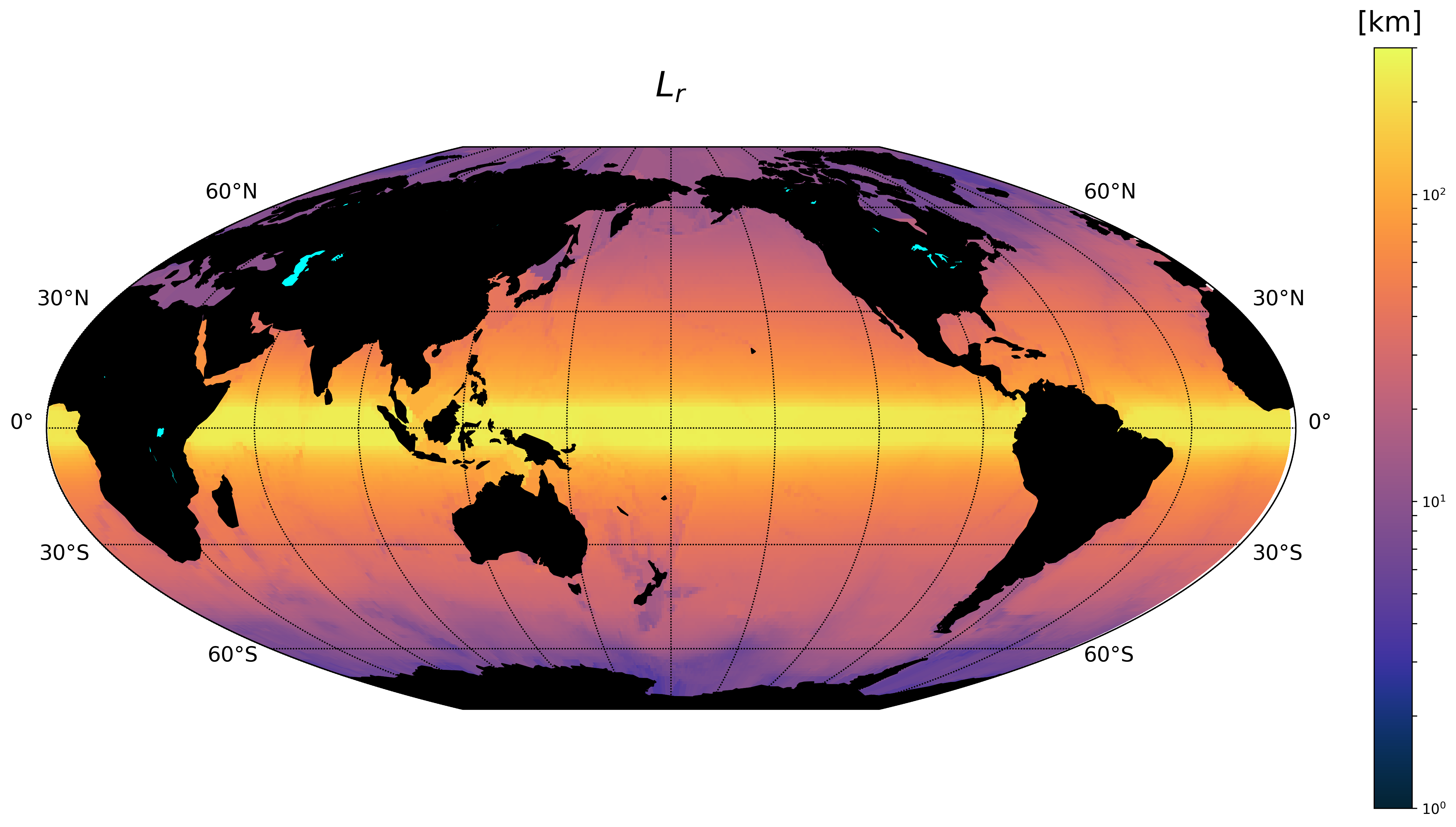
Figure 4. Global First-Baroclinic Rossby Radius of Deformation.

Attention

The decision to calculate areas using boxes instead of polygons reduced the computational time significantly.

Eccentricity

In order to remove elongated features, potentially jets and because eddies are stable coherent structures a condition of eccentricity was imposed. The ellipse eccentricity (\(\epsilon\)) range goes from \(0\) (perfect circle) to 1 (line). Thus the selected value to constrain it represents a semi-minor axis two times smaller than the semi-major axis (\(a=2b\)) or:

\[\epsilon = \left(1-\frac{b^2}{a^2}\right)^\frac{1}{2} \ if \ a<=2b \rightarrow Eddy\ is\ identified\]

or

\[0 \leq \epsilon \leq 0.85\]

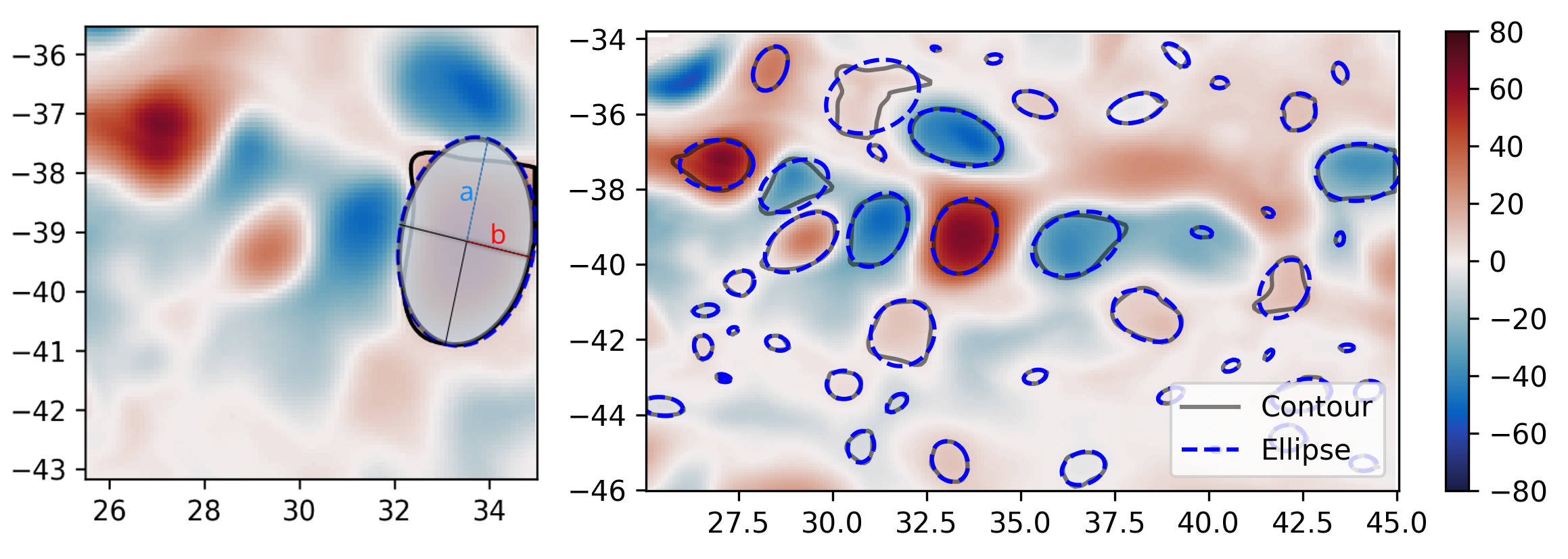
Figure 5. Eddy characterisation based on the eccentricity of the fitted ellipse (blue line).

Gaussian Axis Check

According with 500 detected eddies (Fig. 5), their mean profile can be fitted by a Gaussians and/or paraboloids, however the best fit was found on the Gaussian fit. Additionally, according with diffusion and advection we will expect a decay (Gaussian) instead of an abrupt change (Parabolic). Therefore, to identify an eddy, the data profile of the minor and major axis should have a high coefficient of determination (\(\psi\)) with its optimal fitted gaussian. The interval was define as:

\[0.80 < \psi \leq 1\]

Values around \(1\) represent a exact fitness and the minimum value accepted should be higher than \(0.8\).

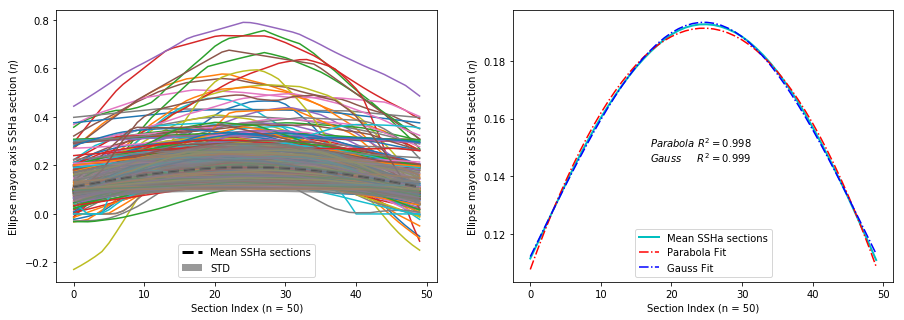
Figure 6. Gaussian and parabolic fit over the average of 500 eddies.

Warning

This criterion potentially will be removed in further versions of the algorithm due to it’s minimal impact over the detected eddies.

Note

After all the previous described criteria the Figure 6 show all identified eddies and their correspondent contour.

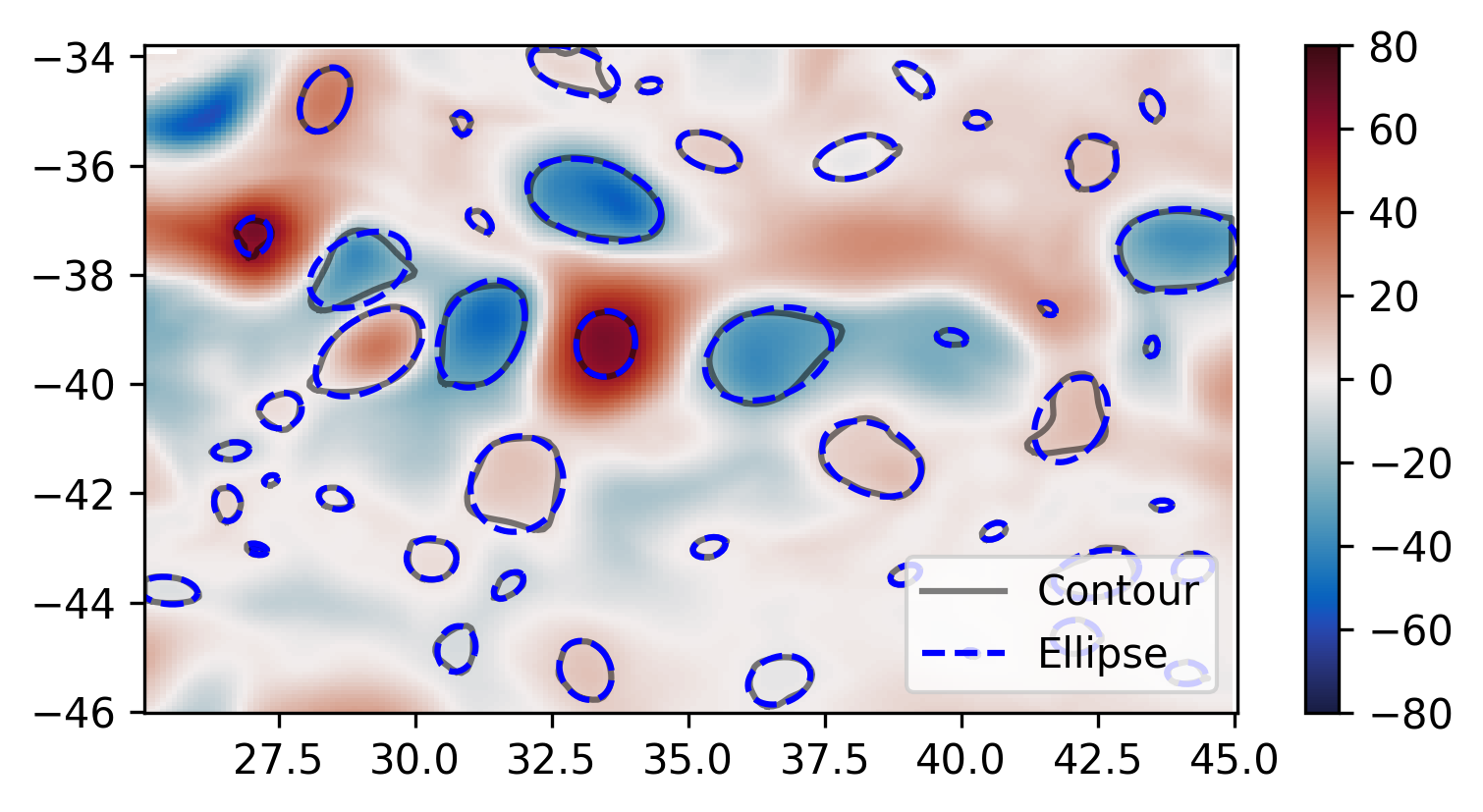
Figure 7. Identified contours using all criteria.

2D Gaussian (Optional)

The fitness of a 2D Gaussian is constrain by the coefficient of determination between the integral of the original field and the fitted field. Additionally, the 2D gaussian fitted must satisfy the same criteria as the eddy identification, otherwise the eddy is discarded.

• Fitted contour area should be within:

\[\frac{A_{contour}}{1.05} \leq A_{2D\ Gaussian} \leq 1.05A_{contour}\]

• 2D gaussian eccentricity should be on range:

\[0 \leq e < 0.95\]

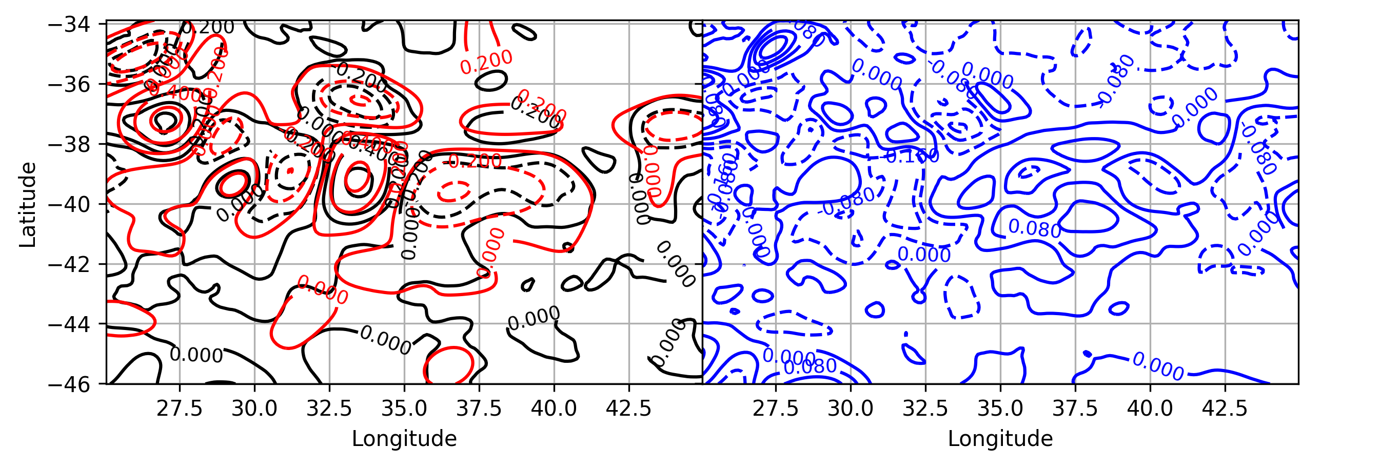
Figure 8. Gaussian fitting. Left panel shows the original field (black line) underlying the reconstructed field (red line). Right panel shows the difference between fields.

Important

If this option is allowed, the condition to identify eddies depends on the fitness of the fitted Gaussian. Which should be within the interval \(0.90 < e_G \leq 1\). Otherwise, the eddy is discarded.

Eddy Contour Replacement

The algorithm correlates vertical contours whenever the level \(l(n-1)\) share their local maxima value and the local coordinates of the maxima with the current analysed level \(l(n)\). This process is only allowed when the contour with level \(l(n)\) passes all the Eddy Identification Criteria

According with the criteria described before, the current algorithm is capable of extracting the eddy signal from Aviso’s dataset.

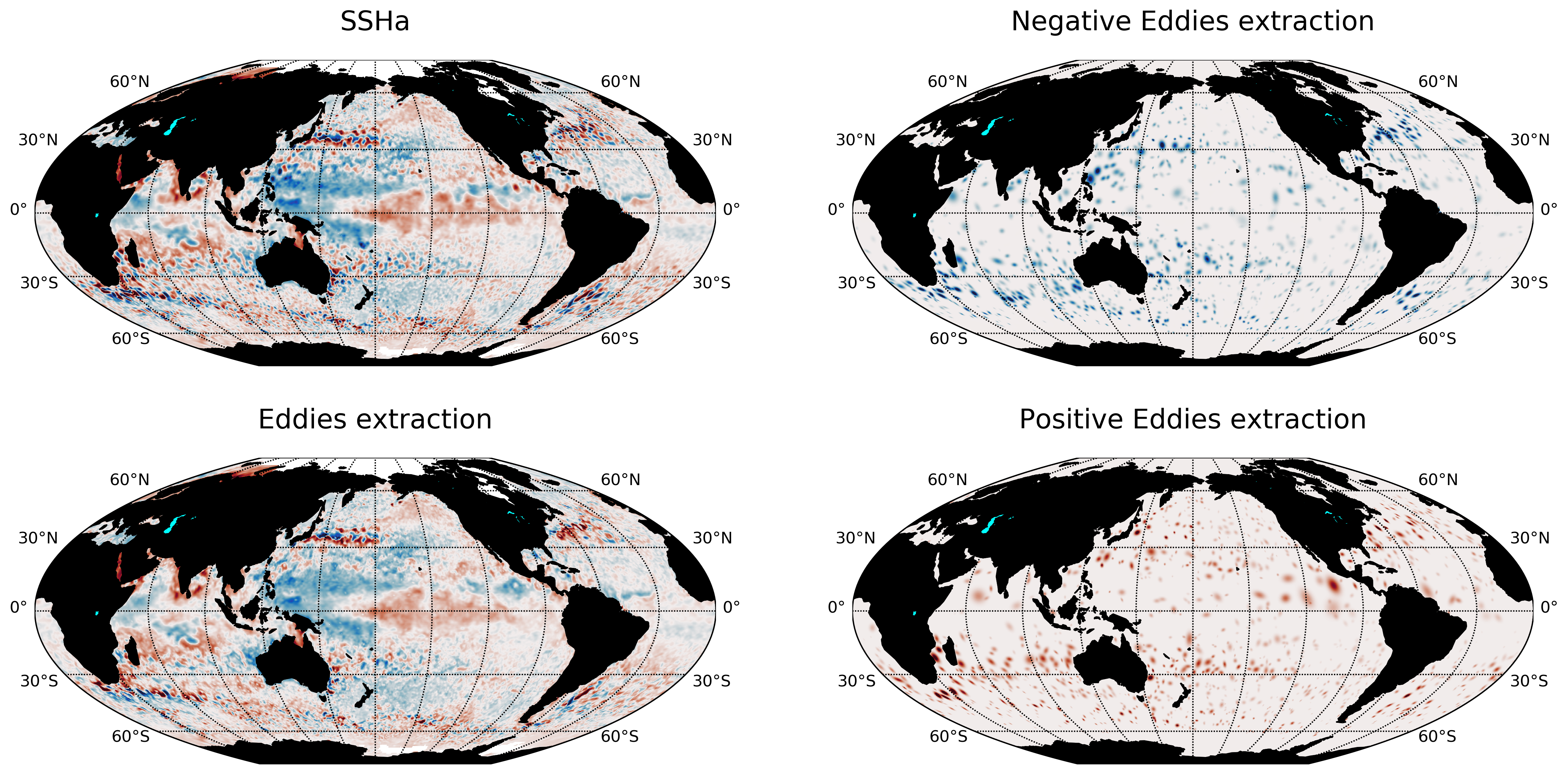
Figure 5. Gaussian fitting in two dimensions to recreate the eddy field. (A) Anti-cyclonic eddy. (B) Cyclonic eddy. (C) Synthetic eddy field. (D) Difference between the original field and the synthetic field [cm].

Eddy Time Tracking

All the transient features are identified in each SLA snapshot, following the eddy identification algorithm, a time tracking is applied: For each eddy feature identified at time \(t\), the features at time \(t+1\) are searched to find an eddy feature inside the close contour or the closest feature within the distance an eddy can displace between two sucessive time frames. This constrain uses the phase speed of a baroclinic Rossby wave, calculated from the Rossby radius of deformation as presented in Celton et. al. [4] and a 180 degree window search using the last peferential direction where the eddy was propagating.

Once a feature at time \(t\) is associated with another feature at time \(t+1\) their amplitude and area is compared. However, this comparison doesn’t avoid the association of eddies cause the nature and purpose of this tracking algorithm.

When global model data is used, the eddies continuity on time is not significative affected, therefore the eddies do not disappear as often as in satellite data (AVISO products). Nonetheless, this tracking algorithm contain an automatic procedure, which allows feature to be reassociated using an user-defined number of time-steps as threshold before terminating the track (This is also related with the traveled distance by the eddy).

Future Methods

Identification

Note

• The phase angle will be implemented in the Beta 0.2 release [5].
• The eddy’s 3D structure will be implemented in the V.1 release.

Time

Note

The 180 degree window and closest feature within the baroclinic Rossby wave speed will be implemented for the next release.